Red Wine Quality Project

Red Wine Quality Project: Full Report

This report outlines the key findings from the Exploratory Data Analysis (EDA) and details the model development process to predict red wine quality.

________________________________________

Part 1: Exploratory Data Analysis (EDA) Insights

The initial analysis was to understand the data's structure, the relationships between different chemical properties, and their collective influence on wine quality.

•Data Integrity : The dataset was loaded successfully and found to be complete, with no missing or null values. This meant no data imputation was necessary.

•Structure ️: The dataset contains 1,599 samples and 12 columns, with 11 being physicochemical features and one being the quality score.

•Quality Distribution : The quality scores are not uniform. They form a normal-like distribution heavily centered around scores of 5 and 6. Wines rated as high quality (7+) or low quality (<5) are significantly less common, creating a class imbalance problem.

•Key Correlations :

oPositive Impact: Alcohol content is the single most positively correlated feature with wine quality. Sulphates and citric acid also show a modest positive correlation.

oNegative Impact: Volatile acidity has the most significant negative correlation; lower levels are a strong indicator of better wine.

________________________________________

Part 2: ️ Model Development and Optimization

To predict whether a wine is "Good" (quality score 7+) or "Bad" (quality score <7), several models and techniques were tested in a systematic way.

Step 1: Data Preparation and Baseline

First, the target variable was simplified by creating a binary column called quality_category (1 for Good, 0 for Bad). The data was then split into an 80% training set and a 20% test set. Initial baseline models (Logistic Regression and Random Forest) were trained, which performed reasonably well but showed difficulty in correctly identifying the minority "Good" wine class due to the data imbalance.

Step 2: ️ Addressing Class Imbalance

Two primary techniques were used to solve the imbalance problem:

1.Class Weighting: A Random Forest model was trained using the class_weight='balanced' parameter. This method automatically adjusts the model's focus, giving more importance to the under-represented "Good" quality wines.

2.SMOTE (Synthetic Minority Over-sampling Technique): This technique was used to generate new, synthetic data points for the minority class in the training set.

Step 3: Feature Scaling

To optimize the performance of certain models, especially Logistic Regression, StandardScaler was applied to the training and test data. This process standardizes each feature by removing the mean and scaling to unit variance.

Step 4: Hyperparameter Tuning

To find the absolute best version of our most promising model (Random Forest), GridSearchCV was employed. This powerful technique systematically tested various combinations of model parameters to find the optimal configuration with the highest F1-score.

________________________________________

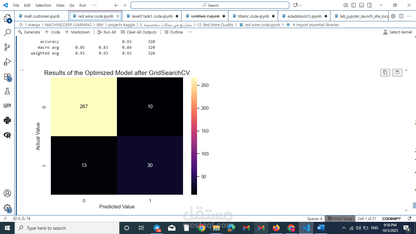
Part 3: Best Performing Model

After all the steps, the best performing model was the tuned Random Forest Classifier that was optimized using GridSearchCV.

This model provided the highest and most balanced performance. It excelled because it combined multiple enhancement strategies:

•It used the class_weight='balanced' parameter to handle imbalance.

•It was trained on scaled data, ensuring feature magnitudes didn't improperly influence results.

•Most importantly, GridSearchCV ensured its internal parameters (n_estimators, max_depth, etc.) were perfectly tuned for this specific dataset.

This final model achieved the best F1-score for the minority "Good" quality class, making it the most reliable and effective predictor among all tested models.