Ames Housing — EDA & Data Cleaning Pipeline

Ames Housing — EDA & Data Cleaning Pipeline

End-to-end exploratory analysis and cleaning of the Ames, Iowa housing dataset, producing a model-ready feature matrix.

Dataset

File Description

AmesHousing.csv Raw source data — 2,930 rows, 82 columns

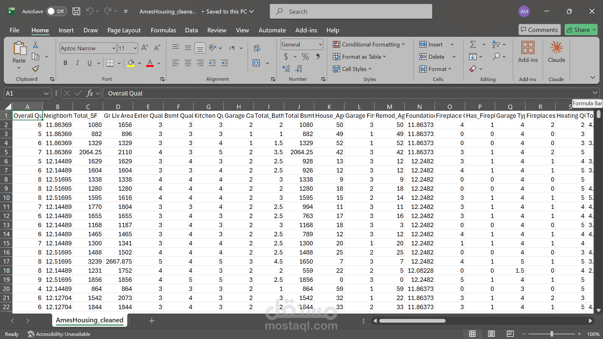
AmesHousing_cleaned.csv Final output — 2,930 rows, 57 columns, features ordered by correlation with SalePrice

Notebook Structure

All work lives in ames_house.ipynb. Run cells top-to-bottom; each section is self-contained.

Section-by-Section Walkthrough

1. Setup

Single cell that imports all dependencies (pandas, numpy, matplotlib, seaborn) and defines DATA_PATH.

Why: Keeping all imports in one place makes dependency management explicit.

2. Load & Inspect

Loads the CSV into df and prints shape, dtype breakdown, and total missing-value count. A .describe().T table gives a statistical overview of all numeric features.

Why: Before touching data, you need a clear picture of what you are working with — dimensions, types, and the scale of the missing-data problem.

3. Reference — Data Dictionary

Markdown reference cells covering every column name, its meaning, and all coded values (quality scales, finish scales, sale codes, etc.).

Why: The Ames dataset uses many short codes (Ex, Gd, TA, GLQ, …). Having the dictionary in the notebook avoids constant look-ups and makes decisions in later steps traceable.

4. Exploratory Data Analysis

4.1 Numeric correlations — heatmap

Full Pearson correlation matrix rendered as a lower-triangle heatmap.

Why: Visually surfaces both the strongest predictors of SalePrice and the clusters of collinear features (which become candidates for pruning in Step 0 of cleaning).

4.2 Top numeric features

Filters to features with |r| > 0.50 against SalePrice and prints them ranked.

Why: Gives a ranked shortlist of numeric signal — used to decide which feature to keep when two are collinear.

4.3 Top categorical features

Computes the correlation ratio (η) for every categorical column against SalePrice.

Why: Pearson correlation only works for numeric variables. The correlation ratio measures how much of the variance in SalePrice is explained by group membership — a model-agnostic signal metric for nominal data.

5. Data Cleaning Pipeline

All steps chain successive copies of the dataframe so the raw df is never mutated.

Step 0 — Drop identifiers & reduce correlated pairs

Drops Order and PID (row identifiers with no predictive signal). Then scans every numeric feature pair: when |r| > 0.70, it drops the feature with the weaker correlation to SalePrice.

Why: Highly collinear features add noise without adding information. Keeping the one more correlated with the target preserves maximum signal. Four pairs were resolved: Garage Cars/Garage Area, Year Built/Garage Yr Blt, Gr Liv Area/TotRms AbvGrd, Total Bsmt SF/1st Flr SF.

Step 1 — Handle missing values

Two strategies applied:

Structural zeros: numeric columns where NaN means "feature not present" (no pool, no garage, no porch) → filled with 0.

Absent categories: all categorical NaN and "NA" strings → replaced with "None" to distinguish "not present" from a genuine unknown.

Why: Deleting rows with nulls would cost ~17% of the dataset (Lot Frontage alone is missing in 490 rows). Treating structural zeros as missing is a data-entry artifact, not a true gap.

Step 2 — Ordinal encoding

Maps ordered categorical features (quality scales, finish levels, exposure ratings) to integers using domain-defined orderings, e.g. Ex=5, Gd=4, TA=3, Fa=2, Po=1, None=0.

Why: Models cannot consume string labels directly, but naive label encoding would imply arbitrary orderings. Using the domain's own ranking (Excellent > Good > Average > …) preserves the true meaning of the ordering.

Step 3 — Cap outliers (IQR method)

For each numeric column, values outside [Q1 − 1.5·IQR, Q3 + 1.5·IQR] are clipped to the boundary. 41 features had outliers capped.

Why: IQR-based capping is robust to the extremes being removed (unlike std-dev methods which are themselves distorted by outliers). Capping, not deletion, preserves every row while preventing extreme values from dominating distance-based or gradient-based models.

Step 4 — Validate

Counts nulls across the entire frame and prints a type breakdown.

Why: Validation after each major transformation is cheap insurance against silent bugs. At this point Lot Frontage still has 490 nulls — intentionally deferred to Step 5 where it receives targeted treatment.

6. Extended Cleaning & Feature Engineering

Step 5 — Targeted imputation

Lot Frontage (16.7% missing): imputed with the median frontage of houses in the same Neighborhood. Street frontage is spatially correlated — houses in the same area share similar lot layouts.

Garage Yr Blt: already removed in Step 0 (collinear with Year Built), so no action needed here.

Why: Filling frontage with a global median would blur the spatial signal. Neighborhood-grouped median is the minimally invasive imputation that preserves geographic structure.

Step 6 — Feature engineering

New features derived then source columns dropped:

New feature Formula Dropped source columns

House_Age Yr Sold − Year Built Year Built, Yr Sold, Mo Sold

Remod_Age Yr Sold − Year Remod/Add Year Remod/Add

Was_Remodeled 1 if remodel year > build year —

Total_SF Total Bsmt SF + 1st Flr SF + 2nd Flr SF individual floor columns

Total_Bath Full + 0.5·Half + Bsmt Full + 0.5·Bsmt Half four bath columns

Total_Porch_SF sum of all porch type areas four porch columns

Has_Pool Pool Area > 0 —

Has_Fireplace Fireplaces > 0 —

Has_Garage Garage Cars > 0 —

Has_2nd_Floor 2nd Flr SF > 0 —

Why: Raw year columns are on an absolute scale that carries no direct signal (a house built in 1972 means nothing without knowing the sale year). Age is the meaningful quantity. Composite area and bath counts reduce dimensionality while concentrating signal — Total_SF ends up as the third-strongest numeric predictor after engineering.

Step 7 — Drop near-zero variance features

Removes any column where ≥ 95% of rows share the same value (21 columns dropped, e.g. Street, Utilities, Heating, Roof Matl).

Why: A feature with no variance cannot predict anything. It only adds noise to distance metrics and wastes coefficients in linear models.

Step 8 — Log-transform skewed features

Applies log1p to numeric features with |skew| > 0.75, excluding binary flags and ordinal-encoded columns. SalePrice is log-transformed separately.

Why: Many area and count features have long right tails (e.g. Misc Val skew = 22). Log transformation compresses the tail, producing more normally distributed residuals and preventing a handful of extreme values from dominating model loss. log1p (log of 1 + x) handles zero values safely.

Step 9 — Smart categorical encoding + weak feature pruning

Two-track encoding to avoid the column explosion from naive OHE (which produced 167 columns):

Track Condition Method

High-cardinality ≥ 6 unique values Target encoding — replace each category with the mean SalePrice for that group (1 column per feature)

Low-cardinality < 6 unique values OHE after consolidating rare categories (< 5% frequency) into "Other"

After encoding, features with |r| < 0.05 against SalePrice are dropped (3 removed: MS SubClass, Land Contour_Other, Lot Config_Other).

Why: Naive OHE of Neighborhood (28 levels) alone would create 27 sparse dummy columns. Target encoding replaces them with a single column that directly encodes the price signal associated with each location — far more compact and just as informative. The leakage note in the notebook is important: in a training pipeline, target means must be computed inside cross-validation folds to prevent overfitting.

Step 10 — Export

Restores SalePrice from log scale back to original dollars (np.expm1), sorts all columns by |correlation with SalePrice| descending, then writes AmesHousing_cleaned.csv.

Why: The log transform on SalePrice was for feature distribution correction, not for the output. Restoring it makes the exported file immediately interpretable. Column ordering by correlation puts the most important features first, matching the convention expected by most downstream modeling workflows.

Final Column Count

Stage Columns

Raw 82

After Steps 0–4 (cleaning) 76

After Step 6 (engineering) 74

After Step 7 (NZV removal) 53

After Step 9 (encoding) 57

Exported 57

Top Predictors in Final Dataset

Ordered by Pearson correlation with SalePrice:

Rank Feature r Notes

1 Overall Qual 0.823 Overall material and finish quality (1–10)

2 Neighborhood 0.769 Target-encoded: mean SalePrice per neighborhood

3 Total_SF 0.735 Engineered: total finished area across all floors

4 Gr Liv Area 0.727 Above-ground living area sq ft

5 Exter Qual 0.709 Exterior quality, ordinal-encoded

6 Bsmt Qual 0.688 Basement quality, ordinal-encoded

7 Kitchen Qual 0.687 Kitchen quality, ordinal-encoded

8 Garage Cars 0.683 Garage capacity

9 Total_Bath 0.663 Engineered: weighted bathroom count

10 Total Bsmt SF 0.649 Total basement square footage

Requirements

pandas

numpy

matplotlib

seaborn

Install with:

pip install pandas numpy matplotlib seaborn