uber data analytics

Project Documentation: Uber Fare Analysis

1. Introduction

This project analyzes Uber ride data to identify key factors that affect fare amounts. The workflow includes data import, cleaning, preprocessing, exploratory data analysis (EDA), visualization, and building predictive machine learning models.

________________________________________

2. Data Import

Imported libraries: pandas, numpy, matplotlib, seaborn, plotly, sklearn

Loaded dataset final_internship_data.csv into a pandas DataFrame

________________________________________

3. Data Cleaning

Removed duplicates to ensure unique records.

Handled missing values by dropping rows with nulls.

Filtered invalid fares:

Removed fares under $0 (not realistic).

Kept fares within a reasonable range ($3 – $30) based on domain knowledge.

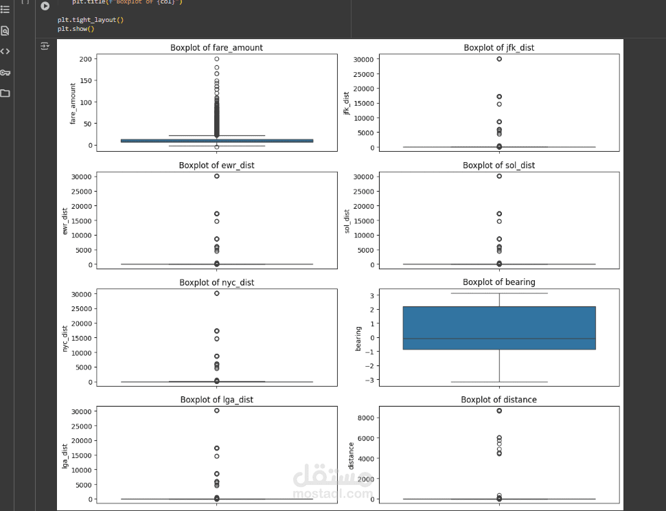
Checked for outliers in numerical columns such as fare_amount and distance.

________________________________________

4. Data Preprocessing

Categorical Features:

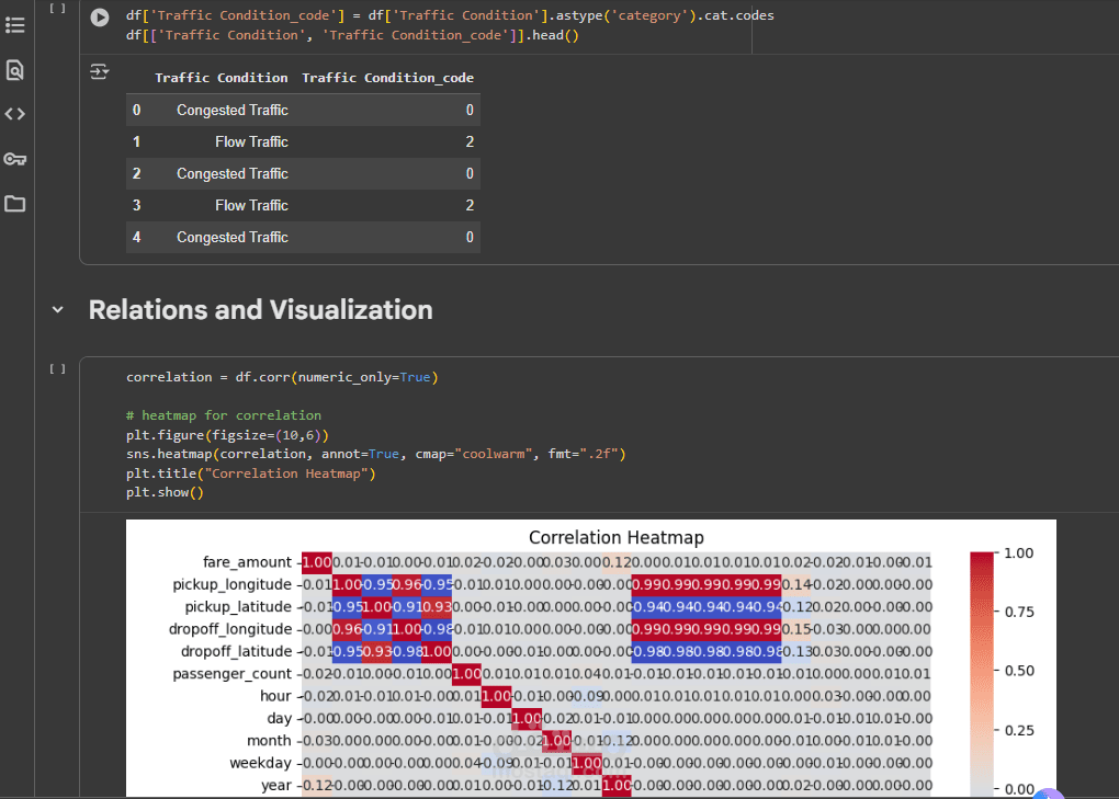
Encoded categorical variables (Weather, Car Condition, Traffic Condition) using One-Hot Encoding.

Numerical Features:

Standardized numerical variables (e.g., distance, year) using StandardScaler.

Target Variable:

fare_amount was separated from the feature set (X) to be predicted by models.

________________________________________

5. Exploratory Data Analysis (EDA)

Key Visualizations & Findings:

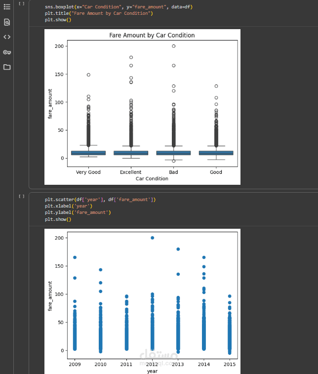
Car Condition vs. Fare

Boxplots showed little to no impact of car condition on fare.

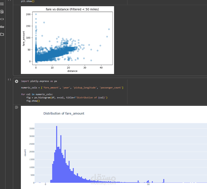
Distance vs. Fare

Scatter plots revealed a strong positive relationship: fares increase with distance.

Passenger Count

Around 70% of rides had only 1 passenger, showing Uber is mostly use individually.

Time of Day

Highest fares occurred around 5 AM, possibly due to airport rides or surge pricing.

Day of Week

Monday had the highest ride requests (first working day after the weekend).

Fare Range

oMost fares fall between $3 and $30.

________________________________________

6. Machine Learning Models

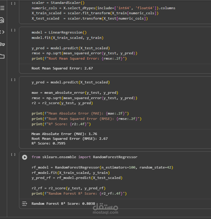
Linear Regression

Built a multiple linear regression model using features like distance, weather, traffic,and passenger count.

Result: Captured trends but limited accuracy due to non-linear relationships and noise in data.

Random Forest Regression

Trained a Random Forest model for better accuracy.

Benefits:

Handles non-linearity better

Less sensitive to outliers.

Higher accuracy compared to linear regression.

________________________________________

7. Model Workflow

Split dataset into training (80%) and testing (20%).

Applied preprocessing (encoding + scaling).

Trained models:

Linear Regression (baseline model).

Random Forest Regressor (improved model).

Evaluated model performance using R² score and Mean Squared Error (MSE).

________________________________________

8. Results

Car condition: not a major factor in fare prediction.

Distance: most significant predictor (strong correlation with fare).

Passenger count: majority are single-passenger rides.

Time and day: Fares peak around 5 AM and requests are higher on Mondays.

Modeling:

Random Forest outperformed Linear Regression in prediction accuracy.

________________________________________

9. Conclusion

Uber fare prediction is primarily influenced by distance and time factors (hour of day, day of week).

Car condition and traffic had minor influence.

Random Forest is a suitable model for predicting fares compared to simple regression.

________________________________________

Mohamed Mahmoud Elramy