Machine Learning course Project

Problem statement:

In netwroking,there are problems of identifying malicous network behavior, so we're trying to build a machine learning model to predict whether the behaviour is an anomoly or normal.

Data Exploration:

We identified the "class" colmn as the target column we're trying to predict, we also looked at the distribution of data and noticed there were many outliers and found the dataset as imbalanced.

Data Preprocessing:

To preprocess the data, we did the following steps:

We applied label encoding to object columns.

from sklearn.preprocessing import LabelEncoder

# transform{protocol, connection_status, service_type, class}

df[df.select_dtypes(include=['object']).columns] = df.select_dtypes(include=['object']).apply(lambda col: LabelEncoder().fit_transform(col.astype(str)))

We split the data, using random seed as 42, to the following: i. Train (70%) ii. Test (15%) iii. Validation (15%)

from sklearn.model_selection import train_test_split

X_train, X_temp, y_train, y_temp = train_test_split(x, y, test_size=0.3, random_state=42)

X_val, X_test, y_val, y_test = train_test_split(X_temp, y_temp, test_size=0.5, random_state=42)

We used an IQR Robust scaler to scale the outliers, which scales the outliers by the interquartile range; we considered using a standard scaler that scales the outliers by subtracting the mean from the data and dividing by the standard deviation but due to the sheer number of outliers the standard scaler wouldn't have been as effective.

from sklearn.preprocessing import RobustScaler

# Automatically select only numeric columns

numeric_cols = X_train.select_dtypes(include='number').columns

# Apply RobustScaler on numeric

scaler = RobustScaler()

X_train[numeric_cols] = scaler.fit_transform(X_train[numeric_cols])

X_val[numeric_cols] = scaler.transform(X_val[numeric_cols])

X_test[numeric_cols] = scaler.transform(X_test[numeric_cols])

X_train = pd.DataFrame(X_train, columns=X_train.columns, index=X_train.index)

X_val = pd.DataFrame(X_val, columns=X_val.columns, index=X_val.index)

X_test = pd.DataFrame(X_test, columns=X_test.columns, index=X_test.index)

We applied an oversampling technique using SMOT to artificially balance the data; we considered an undersampling technique using NearMiss to balance the data but it caused overfitting.

from imblearn.over_sampling import SMOTE

# resample for x_train, y_train only

smote = SMOTE(sampling_strategy='auto', random_state=42, k_neighbors=5)

X_resampled, y_resampled = smote.fit_resample(X_train, y_train)

Feature Engineering:

We decided to choose the 20 most correlated features with the target class through absolute correlation values.

top_20_features = corr_with_target.abs().sort_values(ascending=False).head(20).index

# Keep only top 20 corelated features

X_train_top20 = X_resampled_df[top_20_features]

X_val_top20 = X_val[top_20_features]

X_test_top20 = X_test[top_20_features]

top_20_corr = corr_with_target.loc[top_20_features]

Model Selection and Implementation:

After selecting the most correlated features, we tried different models: KNN, Logistic Regression, Decision Tree, Random Forest, SVM (Soft Margin), and SVM (Hard Margin). We then fine-tuned the parameters for each model to improve performance.

We also applied ensembling techniques to try to get the best out of multiple models and get a more accurate prediction; the ensembling technique we used was "Hard voting".

Model Evaluation:

1. KNN:

We selected the number of neighbors from the range 1 to 21, using only odd values to help improve model accuracy. The model performed best with (1) neighbor, but we avoided this to reduce the risk of overfitting. Instead, we chose 15 neighbors as a more balanced option and the Scores was

Accuracy : 0.9948 Precision : 0.9980 Recall : 0.9965 F1 Score : 0.9973 ROC AUC Score : 0.9753 download

2. Logistic Regression:

In Logistic Regression, we tested lambda values in the range of 1 to 10. The best value was (8), and the performance metrics were:

Accuracy : 0.9568 Precision : 0.9954 Recall : 0.9594 F1 Score : 0.9770 ROC AUC Score : 0.9280 download

The model's performance was not ideal, as the training accuracy was lower than the validation and testing accuracy, which is not typical and suggests possible issues with underfitting or data inconsistencies.

3. Decision Tree:

For the Decision Tree model, we tested max depths of [3, 5, 7, 9, 11]. The model achieved accuracies ranging from 0.95 to 0.9919. The best performance was observed at a depth of (11), and the evaluation scores were:

Accuracy : 0.9929 Precision : 0.9960 Recall : 0.9965 F1 Score : 0.9963 ROC AUC Score : 0.9523 download

Overall, the Decision Tree model outperformed both the KNN and Logistic Regression models.

4. Random Forest:

Among all the models, Random Forest delivered the best overall performance. We experimented with different numbers of estimators and max depths. Specifically, we tested number of estimators [10, 50, 100, 200]. The optimal results were achieved with (50)

The evaluation metrics were: Accuracy : 0.9962 Precision : 0.9975 Recall : 0.9985 F1 Score : 0.9980 ROC AUC Score : 0.9705 download

5. SVM (Soft Margin):

In the Soft Margin SVM, we tried different values of the regularization parameter C from the list [0.001, 0.01, 0.1, 1]. The best value was (1) and the scores were: Accuracy : 0.9867 Precision : 0.9970 Recall : 0.9891 F1 Score : 0.9930 ROC AUC Score : 0.9601 download

The model performance has the same issue as the Logistic Regression model, the training data accuracy was lower than the validation and training accuracy

6. SVM (Hard Margin):

For the Hard Margin SVM, we used larger values of C, specifically [10, 25, 50, 75, 100]. The best performance was achieved with C = (100) and the scores were: Accuracy : 0.9896 Precision : 0.9970 Recall : 0.9921 F1 Score : 0.9945 ROC AUC Score : 0.9616 download

Similar to the Soft Margin SVM, the Hard Margin SVM the training data accuracy was lower than the validation and training accuracy

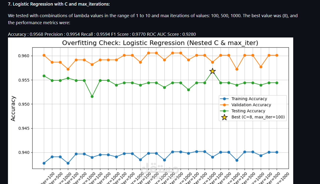
7. Logistic Regression with C and max_iterations:

We tested with combinations of lambda values in the range of 1 to 10 and max iterations of values: 100, 500, 1000. The best value was (8), and the performance metrics were:

Accuracy : 0.9568 Precision : 0.9954 Recall : 0.9594 F1 Score : 0.9770 ROC AUC Score : 0.9280 download

Ensembling (Hard Voting): We applied "Hard voting" as our ensembling technique, the models we used for the technique were [KNN, Logestic reggression, Deision tree, Random forest, SVM (soft margin), and SVM (Hard margin)] The results were very good, we had n_jobs set to -1 so we can parallelise the model,the ensembling had an accuracy of (97.1%), and the scores were: Voting Classifier Accuracy: 0.9706

Previous Trials and attempts

In the process of processing the data and developing the models we tried different methods of data preprocessing to help clean the data and acheive the best performance from all models. Those are the main paths that we followed but pivoted from due to their inefficiency in our current situation.

Scaling Down We tried scaling down the data to match the smaller target class but the data entries were very sparse compared to the number of features leading to inefficient model training and results.

from imblearn.under_sampling import NearMiss

nearmiss = NearMiss(version=1, n_neighbors=3)

X_resampled, y_resampled = nearmiss.fit_resample(X_train, y_train)

X_resampled_df = pd.DataFrame(X_resampled, columns=X_train.columns)

y_resampled_series = pd.Series(y_resampled, name='class')

Standard Scaling Using standard scaling will sabotage the performance due to the sheer amount of outliers. Instead we used Robust scaling to scaling according to the IQR.

Scaling on All Dataset Before Splitting Scaling on the whole dataset affects the performance and leads to overfitting due to the scaling of the training data on metrics from both the test and validation data. That is why we splitted the data before scaling and applied only transform on test and validation

from sklearn.preprocessing import RobustScaler

# Automatically select only numeric columns

numeric_cols = X_train.select_dtypes(include='number').columns

# Apply RobustScaler on numeric

scaler = RobustScaler()

X_train[numeric_cols] = scaler.fit_transform(X_train[numeric_cols])

X_val[numeric_cols] = scaler.transform(X_val[numeric_cols])

X_test[numeric_cols] = scaler.transform(X_test[numeric_cols])

X_train = pd.DataFrame(X_train, columns=X_train.columns, index=X_train.index)

X_val = pd.DataFrame(X_val, columns=X_val.columns, index=X_val.index)

X_test = pd.DataFrame(X_test, columns=X_test.columns, index=X_test.index)

Hot encoding We implemented hot label encoding with a customized approach. After visualizing the qualitative data we deduced that there are some values that have high value counts and some with very low. Therefore, we proceeded with the approach of hot encoding features with high values in a separate column and leaving the remaining ones with low value counts in a separate column called others.

df = pd.get_dummies(df, columns=['protocol'], drop_first=True, dtype=int)

# Create two new features for 'connection_status'

df['connection_status_SF'] = (df['connection_status'] == 'SF').astype(int)

df['connection_status_non_SF'] = (df['connection_status'] != 'SF').astype(int)

# For 'service_type', take top 4 most frequent values and create separate columns

top_4_values = df['service_type'].value_counts().head(4).index

# Create new columns for each of the top 4 service types

for value in top_4_values:

df[f'service_type_{value}'] = (df['service_type'] == value).astype(int)

# Create a new column for the other values (those not in the top 4)

df['service_type_other'] = df['service_type'].apply(lambda x: 1 if x not in top_4_values else 0)

df = df.drop(columns = ['connection_status', 'service_type'])

Conclusion:

In conclusion, we built a machine learning model to detect malicious network behavior by preprocessing an imbalanced dataset, selecting top correlated features, and evaluating several classifiers. Random Forest showed the best individual performance, but our hard voting ensemble—combining multiple models—achieved the highest accuracy at 97.1%. This demonstrates the effectiveness of ensemble methods in anomaly detection and provides a solid foundation for future improvements and real-world applications.