# Mushroom Classification using SVM

This project aims to build a model that can predict whether a mushroom is edible or poisonous based on its various features. The dataset used for this project contains several categorical features describing the physical characteristics of mushrooms.

## Dataset Description

The dataset contains mushrooms classified as either edible (`'e'`) or poisonous (`'p'`). Each mushroom is described by the following features:

- **cap-shape**: bell (`b`), conical (`c`), convex (`x`), flat (`f`), knobbed (`k`), sunken (`s`)

- **cap-surface**: fibrous (`f`), grooves (`g`), scaly (`y`), smooth (`s`)

- **cap-color**: brown (`n`), buff (`b`), cinnamon (`c`), gray (`g`), green (`r`), pink (`p`), purple (`u`), red (`e`), white (`w`), yellow (`y`)

- **bruises?**: bruises (`t`), no (`f`)

- **odor**: almond (`a`), anise (`l`), creosote (`c`), fishy (`y`), foul (`f`), musty (`m`), none (`n`), pungent (`p`), spicy (`s`)

- **gill-attachment**: attached (`a`), descending (`d`), free (`f`), notched (`n`)

- **gill-spacing**: close (`c`), crowded (`w`), distant (`d`)

- **gill-size**: broad (`b`), narrow (`n`)

- **gill-color**: black (`k`), brown (`n`), buff (`b`), chocolate (`h`), gray (`g`), green (`r`), orange (`o`), pink (`p`), purple (`u`), red (`e`), white (`w`), yellow (`y`)

- **stalk-shape**: enlarging (`e`), tapering (`t`)

- **stalk-root**: bulbous (`b`), club (`c`), cup (`u`), equal (`e`), rhizomorphs (`z`), rooted (`r`), missing (`?`)

- **stalk-surface-above-ring**: fibrous (`f`), scaly (`y`), silky (`k`), smooth (`s`)

- **stalk-surface-below-ring**: fibrous (`f`), scaly (`y`), silky (`k`), smooth (`s`)

- **stalk-color-above-ring**: brown (`n`), buff (`b`), cinnamon (`c`), gray (`g`), orange (`o`), pink (`p`), red (`e`), white (`w`), yellow (`y`)

- **stalk-color-below-ring**: brown (`n`), buff (`b`), cinnamon (`c`), gray (`g`), orange (`o`), pink (`p`), red (`e`), white (`w`), yellow (`y`)

- **veil-type**: partial (`p`), universal (`u`)

- **veil-color**: brown (`n`), orange (`o`), white (`w`), yellow (`y`)

- **ring-number**: none (`n`), one (`o`), two (`t`)

- **ring-type**: cobwebby (`c`), evanescent (`e`), flaring (`f`), large (`l`), none (`n`), pendant (`p`), sheathing (`s`), zone (`z`)

- **spore-print-color**: black (`k`), brown (`n`), buff (`b`), chocolate (`h`), green (`r`), orange (`o`), purple (`u`), white (`w`), yellow (`y`)

- **population**: abundant (`a`), clustered (`c`), numerous (`n`), scattered (`s`), several (`v`), solitary (`y`)

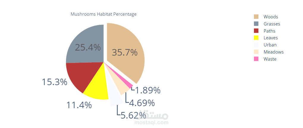
- **habitat**: grasses (`g`), leaves (`l`), meadows (`m`), paths (`p`), urban (`u`), waste (`w`), woods (`d`)

## Exploratory Data Analysis (EDA)

The EDA includes:

- Loading and inspecting the dataset.

- Checking for null values and data types.

- Encoding categorical features using label encoding.

- Visualizing distributions and relationships among features.

- Applying PCA (Principal Component Analysis) for dimensionality reduction.

## Preprocessing

### Label Encoding

All non-numeric features are encoded to numeric values using `LabelEncoder`:

```python

from sklearn.preprocessing import LabelEncoder

mush_encoded = mush.copy()

le = LabelEncoder()

for col in mush_encoded.columns:

mush_encoded[col] = le.fit_transform(mush_encoded[col])

```

### Principal Component Analysis (PCA)

PCA is applied to reduce the dimensionality while retaining most of the variance:

```python

from sklearn.decomposition import PCA

n_components = 12

pca = PCA(n_components=n_components)

mush_encoded_pca = pca.fit_transform(mush_encoded.drop(["class"], axis=1))

```

## Model Training

### Support Vector Machine (SVM)

We use SVM with grid search to find the best hyperparameters:

```python

from sklearn.model_selection import train_test_split, GridSearchCV

from sklearn.svm import SVC

# Split the data

x_train, x_test, y_train, y_test = train_test_split(mush_encoded_pca, mush_encoded["class"].values, random_state=42, test_size=0.25)

# Define the parameter grid

param_grid = {

"C": [0.1, 1, 10, 100],

"gamma": ["scale", "auto", 0.1, 1],

"kernel": ["linear", "rbf", "poly"]

}

# Initialize and perform grid search

svm = SVC(random_state=42)

grid_search = GridSearchCV(svm, param_grid, cv=5)

grid_search.fit(x_train, y_train)

# Best parameters and accuracy

best_svm = grid_search.best_estimator_

print("Best Parameters:", grid_search.best_params_)

print("Test Accuracy after Grid Search: {}%".format(best_svm.score(x_test, y_test) * 100))

```

## Results

- The best parameters found are `{'C': 0.1, 'gamma': 0.1, 'kernel': 'rbf'}`.

- The test accuracy after grid search is approximately `98.86%`.

## Dependencies

- `pandas`

- `numpy`

- `seaborn`

- `matplotlib`

- `plotly`

- `scikit-learn`

To install the required packages, you can use the following commands:

```bash

pip install pandas numpy seaborn matplotlib plotly scikit-learn

```

## Running the Project

1. Clone the repository and navigate to the project directory.

2. Ensure all dependencies are installed.

3. Run the notebook or script containing the code.

## Conclusion

This project successfully builds a model to classify mushrooms as edible or poisonous with high accuracy using SVM and PCA for dimensionality reduction. Further improvements can include testing with different models and additional feature engineering.